In this article we continue the journey through the fundamentals of digital audio. This time – quantization
Introduction
Once we have captured the timing of a sound wave through sampling, we are left with a series of discrete points in time—but these points still possess “infinite” potential values in terms of their height, or amplitude. To translate these physical voltages into a language a computer can actually store, we must perform quantization. This is the process of mapping those continuous, analog measurements onto a fixed scale of digital levels. If sampling is about how often we look at the wave, quantization is about how precisely we measure what we see. It is here that we decide the dynamic range and the “resolution” of our audio, ultimately determining the boundary between a pristine recording and one lost to digital noise.
Quantization
Each sampled amplitude signal value is assigned a numerical value based on its position along a vertical axis divided into discrete levels, presented in binary form.
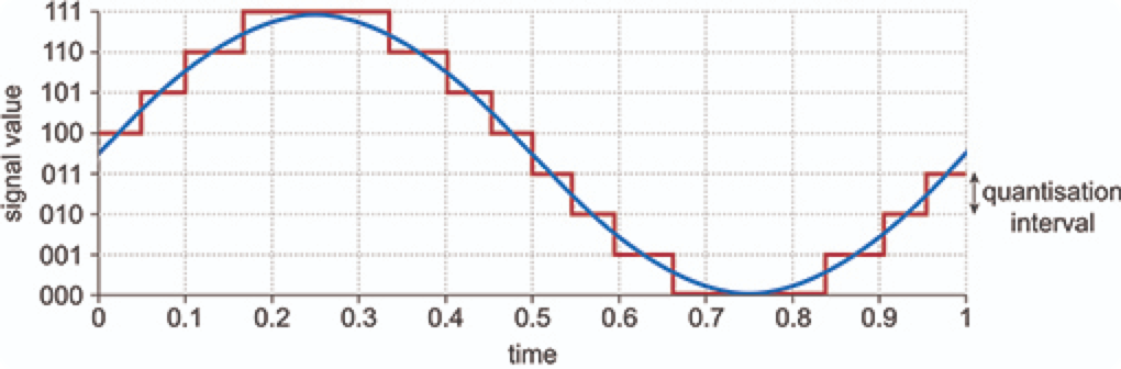
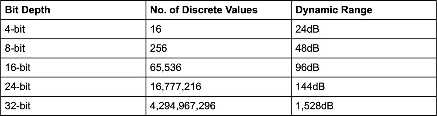
The precision of this step depends on the bit depth (e.g., 16-bit or 24-bit), which defines how many levels are available for representation.
- A 16-bit system provides 2^16 = 65,536216 = 65,536 levels.
- A 24-bit system provides 2^24 = 16,777,216224 = 16,777,216 levels.
Higher bit depth provides greater dynamic range and accuracy.
Dynamic Range
Dynamic Range is the difference between the quietest and loudest sounds that can be represented without distortion.

The ratio of the full scale signal level to the noise floor.
Dynamic Range (dB) = 20 log (2 ^ n) = n x 20 log 2≈ n x 6.0206
n presents here in the formula the nominal number of bits without presentation of quantisizing errors.
The loudest signal in digital audio refers to the maximum amplitude a signal can reach before clipping (distortion caused by exceeding 0 dBFS). Limitations of Fixed-Point Systems:
16-bit PCM:
- Dynamic range: ~96 dB.
- Clipping: Signals exceeding 0 dBFS are permanently distorted.
- Noise floor: Quiet sounds (e.g., whispers at 20 dB) risk being lost in quantization noise when amplified.
24-bit PCM:
- Dynamic range: ~144 dB.
- Clipping: Still occurs at 0 dBFS, requiring careful gain staging.
- Extreme dynamics: Struggles with signals like screams (120 dB) and whispers (20 dB) in the same recording, risking clipping or noise.
Example: A scream recorded at 24-bit may clip if input levels are too high, while amplifying a whisper introduces noise due to the limited bit depth.
32-bit floating point solves this issues:
- Dynamic range: Exceeds 1,500 dB, far beyond physical sound limits.
- No clipping: Signals can temporarily exceed 0 dBFS (e.g., +30 dBFS) without distortion. Peaks are preserved and can be lowered in post-production.
- Ultra-low noise floor: Quiet sounds retain detail even when amplified by +100 dB, avoiding noise floor issues.
Example: A 32-bit float recorder captures a live concert with unpredictable dynamics. Even if the input peaks at +30 dBFS, the file stores the signal intact, allowing engineers to reduce levels later without artifacts.
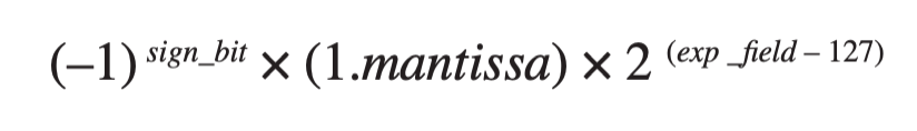
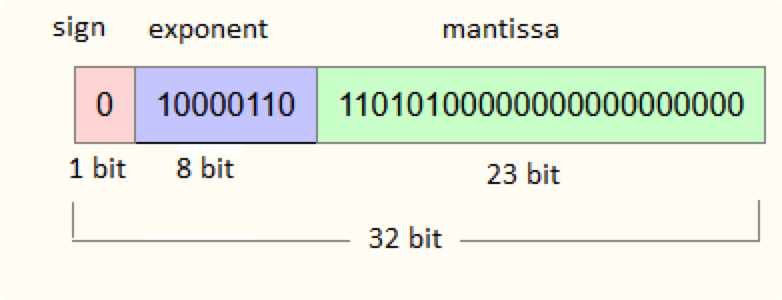
32-bit floating point format
Noise floor
The theoretical minimum noise floor is caused by quantization noise.
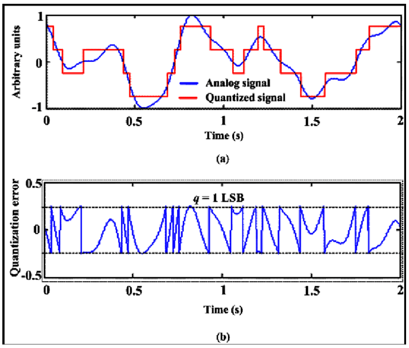
Each sampled amplitude is rounded to the nearest quantization level. This process introduces some error, known as quantization noise or quantization error, which is inversely related to the bit depth.
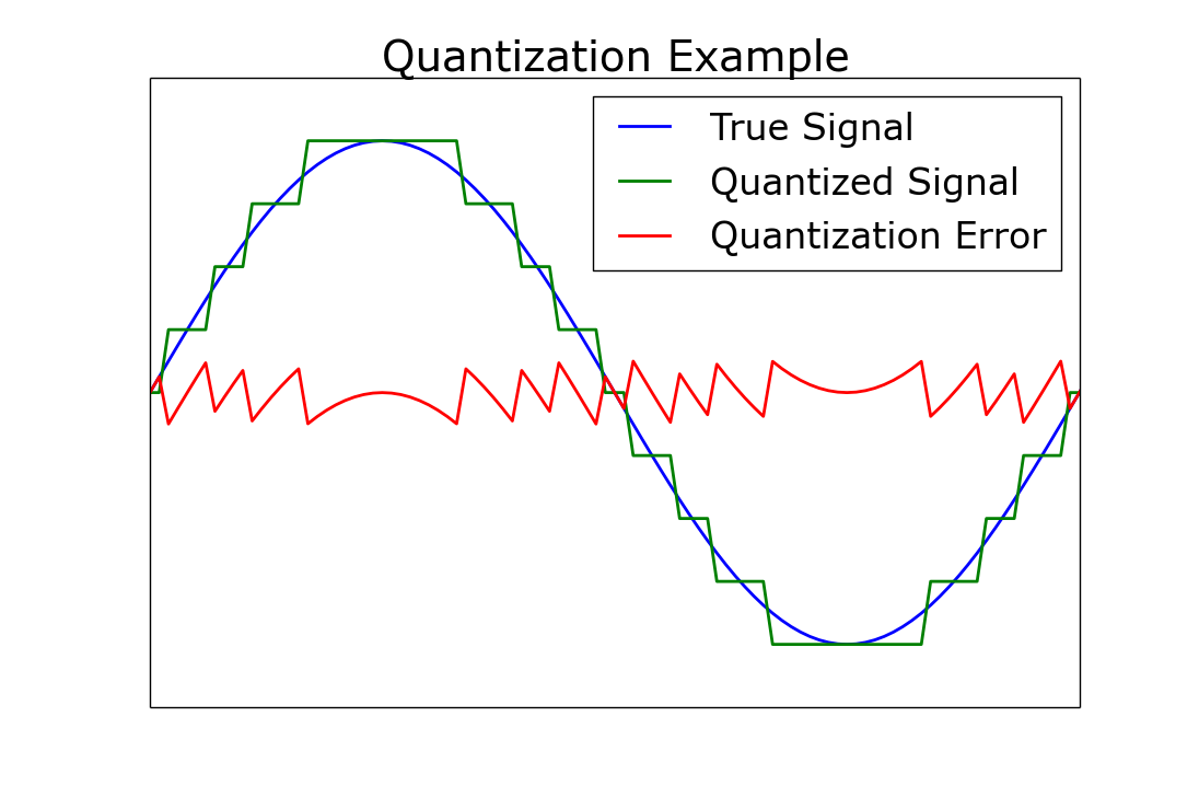
This is usually modeled as a uniform random fluctuation between −1⁄2 LSB and +1⁄2 LSB. (Only certain signals produce uniform random fluctuations, so this model is typically, but not always, accurate). This noise manifests as low-level distortion or hiss in the audio signal.
As the dynamic range is measured relative to the full scale, between peak of the sine wave and the RMS level of this quantization noise in dB FS (Full Scale), both can be estimated with the same formula (though with reversed sign):
DR = 20 log 10 (2^n rsqrt (3/2)) ≈ 6.0206 ^ n + 1.761
The value of n equals the resolution of the system in bits or sometimes the resolution of the system calculated as n-1 bit, because of quantization noise.
The factor rsqrt(3/2) accounts for the RMS value of quantization noise, which is modeled as uniformly distributed noise.
For example, a 16-bit system has a theoretical minimum noise floor of −98.09 dBFS relative to a full-scale sine wave:
DR = 20 log 10 (2^16 x rsqrt(3/2)) ≈ 6.0206 ^ 16 + 1.761 ≈ 98.09
Signal Enhancement & Artifact Mitigation
In any real converter several sophisticated techniques exist to mitigate the detrimental effects of low-level noise and enhance the perceived clarity and fidelity of digital audio, for example dither is added to the signal before sampling. This removes the effects of non-uniform quantization error, but increases the minimum noise floor.
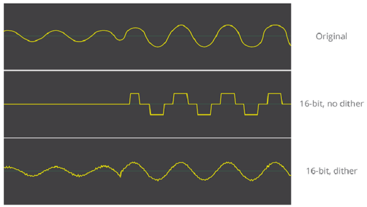
- Dithering stands out as a crucial method employed during bit-depth reduction. When converting from a higher bit depth (e.g., 24-bit) to a lower one (e.g., 16-bit), the process of quantization introduces rounding errors that manifest as audible distortion, particularly at low signal levels. Dithering strategically adds a very small amount of random noise to the audio signal before this quantization stage. This seemingly counterintuitive addition effectively masks the correlated quantization errors, replacing them with a less objectionable, broadband noise floor. The most prevalent form of dither is the
- Triangular Probability Density Function (TPDF), known for its consistent and predictable results across the audio spectrum. For further enhancement
- Noise-Shaped Dither techniques are utilized. These methods go beyond simply masking the noise; they actively shape the frequency spectrum of the dither signal, pushing the majority of the noise energy into higher frequency ranges where human hearing is less sensitive. This clever manipulation significantly improves the perceived signal-to-noise ratio (SNR) in the audible range, resulting in a cleaner and more detailed listening experience, especially for subtle sonic nuances.
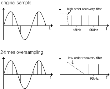
- Oversampling. Improving resolution and SNR, helpful in avoiding aliasing and phase distortion. Oversampling involves multiplying the original sampling rate by an integer factor (e.g., 2x, 4x, or more). For instance, a 44.1 kHz signal can be oversampled to 88.2 kHz or higher. This is achieved by inserting additional “interpolated” samples between the original ones using mathematical algorithms and filtering.
In any real converter several sophisticated techniques exist to mitigate the detrimental effects of low-level noise and enhance the perceived clarity and fidelity of digital audio, for example dither is added to the signal before sampling. This removes the effects of non-uniform quantization error, but increases the minimum noise floor.
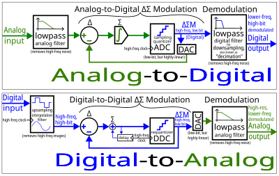
Delta-sigma modulation achieves high quality by utilizing a negative feedback loop during quantization to the lower bit depth that continuously corrects quantization errors and moves quantization noise to higher frequencies well above the original signal’s bandwidth. Subsequent low-pass filtering for demodulation easily removes this high frequency noise and time averages to achieve high accuracy in amplitude, which can be ultimately encoded as pulse-code modulation (PCM).omes the next stage of the signal digitization, quantization.
Summary
Wrapping up, quantization serves as the bridge where the fluid curves of the analog world are finally discretized into the rigid blocks of binary logic. By assigning each sample a specific numerical value based on our chosen bit depth, we solidify the signal’s dynamic foundation, though not without the subtle introduction of quantization error—that ghostly “hiss” we manage through techniques like dither. However, having these measured values is only half the battle; they still need to be formatted into a structure that software can navigate and hardware can transmit. In the next section, we will explore Encoding, where these raw numbers are translated into the final digital bitstream that populates our WAV, FLAC, and MP3 files.